Fast reciprocal square root... in 1997?!
- i76
This article is part of my series on reverse engineering Interstate ‘76, with my current goal being to add a Vulkan renderer to the game. I’m basing this work directly on UCyborg’s patches which include many much-needed fixups to the game, including my own patches for the netcode.
Introduction
Everyone is familiar with the famous fast reciprocal square root function in the Quake 3 source code. And, as noted on Wikipedia, solutions have existed for computing the fast reciprocal square root for many years before that, with perhaps the earliest implementation in 1986.
While I was working on reverse engineering Interstate ‘76, I discovered that Activision had their own implementation in use from at least 1997, and that it shares some similarities with the Quake 3 approach. Interstate ‘76 is based off the Mechwarrior 2 engine – If I had a copy of Mechwarrior 2 (DOS version) on hand, I could confirm if this was present there as well, which would date this technique even earlier! In this post, I’ll explain how it works.
The TL;DR
The approach used in the Mechwarrior 2 engine computes an approximation of the reciprocal
square root using the x87 instruction set at float64 (or double) precision.
It is almost exactly the same as the Quake 3 approach except that the initial guess is computed differently. It still uses Newton-Raphson with a few manual adjustments. The function seems to be accurate within 4 significant digits in the worst case from some brief testing I’ve done.
The initial guess is computed using a Lookup Table (LUT) to obtain mantissa bits. It is best illustrated with the following C++20 code:
uint8_t LUT[256];

void generateLUT()
{
    for (uint32_t i = 0; i < 256; ++i)
    {
        uint64_t const float64bits = (static_cast<uint64_t>(i) | UINT64_C(0x1ff00)) << 0x2d;
        double const d = std::bit_cast<double>(float64bits);
        double const rsqrt = 1.0 / std::sqrt(d);
        uint64_t const u64rsqrt = std::bit_cast<uint64_t>(rsqrt);
        uint32_t const high32bits = static_cast<uint32_t>(u64rsqrt >> 0x20);

        //"round half-up" operation: add 010000000000b (1 << 10): lower bits of mantissa are thrown out.
        //this has the effect of rounding the mantissa within 9 bits
        //using the "round up" rule at the 10-bit mark.
        //likely a bug in the original code: should be 0x800 to correctly round to 8 bits
        uint32_t const high32bits_rounded_up = high32bits + 0x400;
        uint8_t const mantissa_high8bits_only = (high32bits_rounded_up >> 0xc) & UINT32_C(0xFF);

        //store the 8 bits of mantissa remaining
        LUT[i] = mantissa_high8bits_only;
    }
    LUT[0x80] = 0xFF;
}
The exponent of the guess is determined using a formula that operates directly on the exponent field of the input itself.
The LUT has 256 entries, each corresponding a float64 in the range $[0.5,2)$:
- $[0.5,1)$ iterated at a granularity of $0.00390625$ (the first 128 entries)
- $[1,2)$ iterated at a granularity of $0.0078125$ (the second half of the LUT)
Each entry contains the 8 most significant mantissa bits of the reciprocal square root for a
float64corresponding to that entry. It is manually adjusted to create more desirable characteristics when approximating the reciprocal square root of afloat64in the range of $[1,2)$.
Note that the LUT wasn’t precomputed and stored as a static array in the binary – it was generated in the initialization
sequence of the engine. To be honest,
I’m kind of glad – it would have made this analysis a little harder to do!
The code above could easily be made constexpr with a few tweaks.
It compiles to nearly the same code as the original when built with MSVC 2019.
The actual fast reciprocal square root function computes the result as follows:
- Compute an initial guess for the result:
- the exponent bits for the initial guess is determined through a formula that involves only addition and division by 2 (bit shift)
- the mantissa bits for the initial guess is determined using the lookup table
orthese values together to form a validfloat64– this is the guess
- Perform one iteration of Newton-Raphson on the initial guess
- Multiply the result by the constant $1.00001$
Below is my own reverse engineered C++20 version of this function:
double i76_rsqrt(double const scalar)
{
    uint64_t const scalar_bits = std::bit_cast<uint64_t>(scalar);

    uint8_t const index = (scalar_bits >> 0x2d) & 0xff;

    //LUT[index] contains the 8 most significant bits of the mantissa, rounded up.
    //Treat all lower 44 bits as zeroed out
    uint64_t const mantissa_bits = static_cast<uint64_t>(LUT[index]) << 0x2c;

    //Exponent bits are calculated based on the formula in the article
    uint64_t const exponent_bits = ((0xbfcUL - (scalar_bits >> 0x34)) >> 1) << 0x34;

    //exponent_bits have form 0xYYY00000 00000000
    //mantissa_bits have form 0x000ZZ000 00000000
    //so combined, we have    0xYYYZZ000 00000000 -- a complete float64 for the guess
    uint64_t const combined_bits = exponent_bits | mantissa_bits;

    auto const initial_guess = std::bit_cast<double>(combined_bits);

    auto const half_initial_guess = initial_guess * 0.5;
    auto const initial_guess_squared = initial_guess * initial_guess;

    //One iteration of Newton-Raphson
    auto const newton_raphson = (3.0 - (scalar * initial_guess_squared)) * half_initial_guess;

    //post-hoc fixup
    auto const fixup = newton_raphson * 1.00001;

    return fixup;
}
»> Compiler Explorer
When compiled for x86 using only x87 instructions and -Ofast on Clang 11, it produces similar assembly to the original with a few differences.
Patched version of game with screenshots
So, I went ahead and replaced this with a much more accurate rsqrt in I'76. Here’s a comparison between the original and both versions, with differences marked using
purple:

Hardly any difference! The original version of the code was definitely “good enough” for what it needed to do.
The Long Version
Foreword
You know, back when I first started delving into reverse engineering I'76 ten years ago, tools like Ghidra weren’t available. The state of the art was probably IDA Pro, a tool suite that while reasonably priced for what it did, was way out of the price range for me, a third year undergraduate student. Sure, pirating it was an option, but if you wanted to do things the honest way and on a budget, it was hard to do better than Ollydbg, a free debugger and disassembler for 32-bit x86. Now, ten years later, the landscape looks radically different. There are so many fantastic tools available for doing this kind of thing, and it has never been easier to mod your favourite games as a result.
Introduction
I first discovered the code when identifying functions in the startup sequence of nitro.exe using Ghidra. Some fairly
normal initialization code, then I came across this function that populates a LUT using, seemingly, one byte from the result of a 1.0/sqrt(x) on a float64.
Below is the decompiled version of the function as provided by Ghidra:
void generate_weird_lut(void)
{
  int uVar1;
  double local_10;
  double var1;

  uVar1 = 0;
  do {
    var1._4_4_ = (int)((ulonglong)
      (1.0 / SQRT((double)((ulonglong)((uVar1 | 0x1ff00U) << 0xd) << 0x20))) >> 0x20);
    global_lut[uVar1] = (byte)(var1._4_4_ + 0x400 >> 0xc);
    uVar1 = uVar1 + 1;
  } while (uVar1 < 0x100);
  global_lut[128] = 0xff;
  return;
}
Ghidra did pretty well here, except the cast to double, which is closer to a bitwise cast than a static_cast:
Assembly listing for generate_weird_lut
0049AF60 | 83EC 10                  | sub esp,10
0049AF63 | 33C0                     | xor eax,eax
0049AF65 | 894424 00                | mov dword ptr ss:[esp],eax
0049AF69 | 8BC8                     | mov ecx,eax
0049AF6B | 81C9 00FF0100            | or ecx,1FF00
0049AF71 | C1E1 0D                  | shl ecx,D
0049AF74 | 894C24 04                | mov dword ptr ss:[esp+4],ecx
0049AF78 | DD4424 00                | fld st(0),qword ptr ss:[esp]
0049AF7C | D9FA                     | fsqrt
0049AF7E | DC3D A0504C00            | fdivr st(0),qword ptr ds:[4C50A0]
0049AF84 | DD5C24 08                | fstp qword ptr ss:[esp+8],st(0)
0049AF88 | 8B5424 0C                | mov edx,dword ptr ss:[esp+C]
0049AF8C | 81C2 00040000            | add edx,400
0049AF92 | C1FA 0C                  | sar edx,C
0049AF95 | 8890 80B15F00            | mov byte ptr ds:[eax+5FB180],dl
0049AF9B | 40                       | inc eax
0049AF9C | 3D 00010000              | cmp eax,100
0049AFA1 | 7C C6                    | jl nitro.49AF69
0049AFA3 | C605 00B25F00 FF         | mov byte ptr ds:[5FB200],FF
0049AFAA | 83C4 10                  | add esp,10
0049AFAD | C3                       | ret
Only one other function referenced this lookup table, and the code was almost incomprehensible at first glance:
float10 weird_function(double param_1)
{
  uint uVar1;
  float10 fVar2;

  uVar1 = (0xbfc - (param_1._4_4_ >> 0x14) >> 1) << 0x14 |
          (uint)global_lut[param_1._4_4_ >> 0xd & 0xff] << 0xc;
  fVar2 = (float10)(double)((ulonglong)uVar1 << 0x20);
  return ((float10)double_3.0 - fVar2 * fVar2 * (float10)param_1) *
         (float10)(double)((ulonglong)uVar1 << 0x20) * (float10)double_0.5 *
         (float10)double_approx_1.00001;
}
Again Ghidra did a good job here, except for the cast to double – the pseudo-C code above is basically a more
readable version of the assembly listing.
Assembly listing for weird_function
0049C310 | 8B4C24 08                | mov ecx,dword ptr ss:[esp+8]
0049C314 | BA FC0B0000              | mov edx,BFC
0049C319 | C1E9 14                  | shr ecx,14
0049C31C | 8B4424 08                | mov eax,dword ptr ss:[esp+8]
0049C320 | C1E8 0D                  | shr eax,D
0049C323 | 2BD1                     | sub edx,ecx
0049C325 | D1EA                     | shr edx,1
0049C327 | 25 FF000000              | and eax,FF
0049C32C | DD4424 04                | fld st(0),qword ptr ss:[esp+4]
0049C330 | C1E2 14                  | shl edx,14
0049C333 | 8A80 80B15F00            | mov al,byte ptr ds:[eax+5FB180]
0049C339 | C1E0 0C                  | shl eax,C
0049C33C | 33C9                     | xor ecx,ecx
0049C33E | 0BD0                     | or edx,eax
0049C340 | 894C24 04                | mov dword ptr ss:[esp+4],ecx
0049C344 | 895424 08                | mov dword ptr ss:[esp+8],edx
0049C348 | DD4424 04                | fld st(0),qword ptr ss:[esp+4]
0049C34C | DCC8                     | fmul st(0),st(0)
0049C34E | DD4424 04                | fld st(0),qword ptr ss:[esp+4]
0049C352 | D9C9                     | fxch st(0),st(1)
0049C354 | DECA                     | fmulp st(2),st(0)
0049C356 | DC0D 68115000            | fmul st(0),qword ptr ds:[501168]
0049C35C | D9C9                     | fxch st(0),st(1)
0049C35E | DC2D 60115000            | fsubr st(0),qword ptr ds:[501160]
0049C364 | DEC9                     | fmulp st(1),st(0)
0049C366 | DC0D 70115000            | fmul st(0),qword ptr ds:[501170]
0049C36C | C3                       | ret
Bit shifts, floats being treated like integers, and other interesting things abound! It could be what I was suspecting, a fast reciprocal square root function, but maybe it was just a small piece of code used for something else. Not wanting to jump to conclusions, I decided to study it a bit more. A good place to start, I figured, would be to see how this mysterious function was used. I found fragments of code like this all over the place:
//...
fVar2 = (float)*param_2 - (float)*param_1;
fVar4 = (float)param_2[1] - ((float)param_1[1] - 2.0);
fVar3 = (float)param_2[2] - (float)param_1[2];
fVar8 = weird_function((double)(fVar3 * fVar3 + fVar4 * fVar4 + fVar2 * fVar2));
fVar1 = (float)fVar8;
fVar2 = fVar2 * fVar1;
fVar3 = fVar3 * fVar1;
//...
“Wow, that sure looks like it’s computing the squared length of a 3D vector,” I thought to myself.
If weird_function was being called on the results of squared vector lengths, it’s almost certain it’s being used in vector normalization. Indeed,
in the fragment of code above, you can see some of the vector components being multiplied by the result.
Wanting to play with some new tools, I gave Cutter a try with its emulation facilities to run the machine code directly, but unfortunately
couldn’t figure out how to get it to show the ST(i) registers during execution. So I moved on to
x64dbg, a modern debugger heavily inspired by Ollydbg.
I fired up x64dbg and set a breakpoint for right after where the function where the LUT gets generated is called, then ran it.
Once execution reached the breakpoint, I immediately replaced the instruction pointer to the start of our weird_function:

Seeing where the argument was expected, I figured why not try evaluating the value 2.0? So, I passed it in
and ran the function to completion:

Indeed, after running the function, 0.7071... was sitting in ST(0). That’s 1/sqrt(2) accurate to 4 significant digits.
“OK fine,” I thought, “let’s try out some other values too, just to be sure.”
So, I went ahead and tried out 100, 4, 64, 0.5, and 1.2345:
Trying with 100: 
With 4: 
With 64: 
With 0.5: 
Finally, with 1.2345: 
In each case, the result seemed to be accurate within 4 to 6 significant digits.
“That’s it. I’m convinced!” I said out loud, “…but what the hell is it actually doing?!”
The next step, I figured, would be to decompile it to C++ to help analyze it a bit easier. This would be a manual process guided by Ghidra’s own decompilation, which did a pretty good job, considering. I wanted to compare it against a correctly rounded reciprocal square root to sample what the error was across the board.
First, the C++20 version of the LUT generator:
uint8_t LUT[256];

void generateLUT()
{
    for (uint32_t i = 0; i < 256; ++i)
    {
        uint64_t const float64bits = (static_cast<uint64_t>(i) | UINT64_C(0x1ff00)) << 0x2d;
        double const d = std::bit_cast<double>(float64bits);
        double const rsqrt = 1.0 / std::sqrt(d);
        uint64_t const u64rsqrt = std::bit_cast<uint64_t>(rsqrt);
        uint32_t const high32bits = static_cast<uint32_t>(u64rsqrt >> 0x20);

        //"round half-up" operation: add 010000000000b (1 << 10): lower bits of mantissa are thrown out.
        //this has the effect of rounding the mantissa within 9 bits
        //using the "round up" rule at the 10-bit mark.
        //likely a bug in the original code: should be 0x800 to correctly round to 8 bits
        uint32_t const high32bits_rounded_up = high32bits + 0x400;
        uint8_t const mantissa_high8bits_only = (high32bits_rounded_up >> 0xc) & UINT32_C(0xFF);

        //store the 8 bits of mantissa remaining
        LUT[i] = mantissa_high8bits_only;
    }
    LUT[0x80] = 0xFF;
}
Assembly comparison
If you compile this for 32-bit with MSVC 2019, x87 only, and /fp:fast you will get nearly identical assembly to what is in I'76:
Assembly listing comparison between the original and C++20 version of generateLUT
; Original I'76                     |   ;New code, MSVC 2019, x86-Release with /arch:IA32 /fp:fast
                                    |   ; /Oy /O2 /Ot /Ob2 /Oi
sub esp,10                          |   sub         esp,14h
                                    |   fld1
xor eax,eax                         |   xor         ecx,ecx
mov dword ptr ss:[esp],eax          |   mov         eax,ecx
mov ecx,eax                         |   mov         dword ptr [esp],0
or ecx,1FF00                        |   shl         eax,0Dh
shl ecx,D                           |   or          eax,3FE00000h
mov dword ptr ss:[esp+4],ecx        |   mov         dword ptr [esp+4],eax
fld st(0),qword ptr ss:[esp]        |   fld         qword ptr [esp]
fsqrt                               |   fsqrt
fdivr st(0),qword ptr ds:[4C50A0]   |   fdivr       st,st(1)
fstp qword ptr ss:[esp+8],st(0)     |   fstp        qword ptr [esp+8]
mov edx,dword ptr ss:[esp+C]        |   mov         eax,dword ptr [esp+0Ch]
add edx,400                         |   add         eax,400h
sar edx,C                           |   shr         eax,0Ch
mov byte ptr ds:[eax+5FB180],dl     |   mov         byte ptr LUT (0B66678h)[ecx],al
inc eax                             |   inc         ecx
cmp eax,100                         |   cmp         ecx,100h
jl nitro.49AF69                     |   jb          generateLUT+7h (0B61827h)
                                    |   fstp        st(0)
mov byte ptr ds:[5FB200],FF         |   mov         byte ptr ds:[0B666F8h],0FFh
add esp,10                          |   add         esp,14h
ret                                 |   ret
This is acceptable. The only real difference is the constant 1.0 is obtained via fld1 rather than a memory reference, and the function cleans it off the x87 stack before returning (this is
a requirement imposed by the cdecl calling convention). Comparing the LUT generated here with the one visible in x64dbg yielded identical results, so I was confident I got this right. Now I could actually pick this apart a bit.
You might have noticed that the LUT could have been computed entirely at compile time, or even just stored as a static array in the executable. I’m glad that Visual C++ 6.0 wasn’t that smart, because it would have made this a fair bit harder to do!
Some basic analysis of the LUT
The 256-entry LUT looks like this:
0x00:  6a 68 67 66 64 63 62 60 5f 5e 5c 5b 5a 59 57 56 55 54 53 52 50 4f 4e 4d 4c 4b 4a 49 48 47 46 45
0x20:  44 43 42 41 40 3f 3e 3d 3c 3b 3a 39 38 37 36 35 34 34 33 32 31 30 2f 2f 2e 2d 2c 2b 2a 2a 29 28
0x40:  27 27 26 25 24 24 23 22 21 21 20 1f 1f 1e 1d 1c 1c 1b 1a 1a 19 18 18 17 16 16 15 15 14 13 13 12
0x60:  11 11 10 10 0f 0e 0e 0d 0d 0c 0c 0b 0a 0a 09 09 08 08 07 07 06 05 05 04 04 03 03 02 02 01 01 00
0x80:  ff fe fc fa f8 f6 f4 f2 f0 ef ed eb e9 e8 e6 e4 e2 e1 df de dc da d9 d7 d6 d4 d3 d1 d0 ce cd cb
0xa0:  ca c8 c7 c5 c4 c3 c1 c0 bf bd bc bb b9 b8 b7 b6 b4 b3 b2 b1 b0 ae ad ac ab aa a8 a7 a6 a5 a4 a3
0xc0:  a2 a1 a0 9f 9e 9c 9b 9a 99 98 97 96 95 94 93 92 91 90 8f 8f 8e 8d 8c 8b 8a 89 88 87 86 85 85 84
0xe0:  83 82 81 80 7f 7f 7e 7d 7c 7b 7a 7a 79 78 77 76 76 75 74 73 73 72 71 70 70 6f 6e 6d 6d 6c 6b 6a
As you can see, there is a discontinuity between 0x7f and 0x80, where it jumps from 00 to ff.
I made a spreadsheet to see how this compares to the “precise” result and ended up seeing that the numerical error actually forms a repeating pattern when viewed on a log scale, which at the time I thought was interesting. We’ll see why this is the case later.
I tried out the decompiled version of the code by sampling inputs and comparing them with the correctly rounded “ground truth” result. The code appears to give about 4 significant digits of precision in the worst case, sometimes providing 6 or more. Not bad at all!
But how’s this thing actually work?
IEEE-754 float64 refresher
Before we go down the numerical analysis path – a quick refresher on IEEE-754 float64 (or double precision) representations
is due.
A float64 value is a 64-bit datatype of the following form, where the sign bit is the most significant bit:
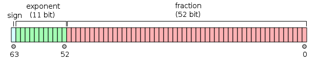
Image courtesy of Wikipedia
Conceptually, you can think of a float64 like you would a number written in scientific notation,
except in base 2 instead of base 10.
There are certain special cases of this format that, for our purposes, we can completely ignore for our analysis.
We assume, because we’re dealing with an approximation, that the input is:
- non-
NaN - non-
InF(i.e. finite) - normal (i.e. not denormal/subnormal)
- positive (i.e., the sign bit is zero)
These assumptions simplify the math and handle the vast majority of use cases that this function would be used for. Remember: this thing is supposed to be a fast approximation, not perfect.
There are just two more things to point out before we proceed. Given a float64 $v$ conforming to our assumptions:
- The 11-bit exponent for $v$ is stored biased by the value $1023$ in the exponent field. This means to get the true exponent, you need to subtract it by $1023$
- The mantissa for $v$ is actually a 53-bit value. The lower 52-bits are as they appear in the mantissa field, and the most significant bit is implicitly $1$
For example, the value $-3.625$ is represented as a float64 as follows: first, $-3.625 = -2^1(1 + 0.8125)$. Therefore the unbiased exponent is $1$, and
the biased exponent is $1 + 1023 = 1024$. The fractional part of the mantissa (lower 52 bits) is 0.8125, as we exclude the implicit leading $1$.
We turn that into a 52-bit integer for the field by multiplying it by $2^{52}$. Finally, the sign bit is $1$ because the quantity is negative:
1     10000000000 1101000000000000000000000000000000000000000000000000
^     ^           ^
sign  exponent    mantissa
In hexadecimal notation, this is written as 0xc00d000000000000. float64 is kind of nice because the mantissa starts on a 4-bit (or nibble) boundary, so it’s easy to see what the fractional
part of the mantissa is just by looking at the hexadecimal readout.
Working with values this way is a little cumbersome, so let us introduce some notation to make working with float64s a little easier.
Notation
We can represent an IEEE-754 value $v$ that conforms to our assumptions as follows:
\[\newcommand{\fexp}{\mathit{exp}} \newcommand{\ffrac}{\mathit{frac}} \mathrm{fl}[v] = 2^\fexp(1 + \ffrac)\]where $\mathrm{fl}[v] \in \mathbb{R}$ is the real floating point value, $\fexp \in \mathbb{Z}$ is the unbiased exponent, and $\ffrac \in \mathbb{R}$ is the fractional part of the mantissa, $0 \leq \ffrac < 1$.
This is a common notation used in many numerical analysis papers and will help along our exploration.
Note that this is a “one way” mapping from floating point values to reals. Taking an arbitrary real number and approximating it with a float64 requires certain conditions to be met.
The fast reciprocal square root function i76_rsqrt
Onto the math. Recall what our decompiled i76_rsqrt function looks like:
float10 i76_rsqrt(double param_1)
{
  uint uVar1;
  float10 fVar2;

  uVar1 = (0xbfc - (param_1._4_4_ >> 0x14) >> 1) << 0x14 |
          (uint)global_lut[param_1._4_4_ >> 0xd & 0xff] << 0xc;
  fVar2 = (float10)(double)((ulonglong)uVar1 << 0x20);
  return ((float10)double_3.0 - fVar2 * fVar2 * (float10)param_1) *
         (float10)(double)((ulonglong)uVar1 << 0x20) * (float10)double_0.5 *
         (float10)double_approx_1.00001;
}
Now we’ll take this function apart piece by piece to figure out what the magic is. The general algorithm is as follows:
We’ll address each step in order.
Forming the initial guess
The initial guess is also a float64. Since it has three components (sign, biased exponent, and mantissa),
wouldn’t it be nice if you could solve for each of them independently?
As it turns out, it is possible do just that! We’ll start with an exact floating point decomposition of the reciprocal square root
and then start simplifying things to create an approximation of it.
The Sign bit
First, observe that the sign bit of the result has to be 0, which denotes a non-negative number in IEEE-754. This is because the reciprocal square root is always a positive value. So that one was easy! :)
0     ?????🔒????? ??????????????????????????🔒?????????????????????????
^     ^           ^
sign  exponent    mantissa
Hey, it’s a start!
The Exponent
Now onto solving for the exponent field.
float10 i76_rsqrt(double param_1)
{
  uint uVar1;
  float10 fVar2;

  uVar1 = (0xbfc - (param_1._4_4_ >> 0x14) >> 1) << 0x14 |
          (uint)global_lut[param_1._4_4_ >> 0xd & 0xff] << 0xc;
  fVar2 = (float10)(double)((ulonglong)uVar1 << 0x20);
  return ((float10)double_3.0 - fVar2 * fVar2 * (float10)param_1) *
         (float10)(double)((ulonglong)uVar1 << 0x20) * (float10)double_0.5 *
         (float10)double_approx_1.00001;
}
One way to figure out what the exponent should be in our float64 is to take the floor of the base-2 logarithm of the value, denoted $\lg$:
Now, $\fexp/2$ may not be an integer, therefore some odd/even analysis is in order.
Note the following:
\begin{aligned}&1 \leq 1 + \ffrac < 2 \\ \implies& 0 \leq \lg(1 + \ffrac) < 1 \\ \implies& 0 \leq \frac{\lg(1 + \ffrac)}{2} < \frac{1}{2} \tag{1}\end{aligned}Odd case
Assume that $\fexp$ is odd:
\begin{aligned}&\floor{-\frac{\fexp}{2} - \frac{\lg(1 + \ffrac))}{2}} \\ =&\floor{\floor{-\frac{\fexp}{2}} + \frac{1}{2} - \frac{\lg(1 + \ffrac))}{2}} \\ =&\floor{-\frac{\fexp}{2}}\qquad\qquad\qquad\qquad(\text{from }(1))\\ =&-\frac{\fexp}{2} - \frac{1}{2}\qquad\qquad\qquad(\fexp\text{ is odd}) \\ =&-\frac{\fexp + 1}{2}\end{aligned}Note that $\fexp + 1$ is even, and therefore $-\dfrac{\fexp + 1}{2}$ is a valid exponent for IEEE-754.
Even cases
Now assume that $\fexp$ is even. Therefore $\dfrac{\fexp}{2}$ is indeed an integer. However, there are two cases to deal with: $\ffrac = 0$ and $\ffrac \neq 0$. If $\ffrac = 0$ then:
\[\floor{- \frac{\fexp}{2} - \frac{\lg(1 + \ffrac))}{2}} \\[0.2em] =-\frac{\fexp}{2}\]On the other hand, if $\ffrac \neq 0$ then :
\[\floor{- \frac{\fexp}{2} - \frac{\lg(1 + \ffrac))}{2}} \\[0.2em] =-\frac{\fexp}{2} - 1 \\[0.2em] =-\frac{\fexp + 2}{2}\]Putting it together
Let’s recap. Let $r_\fexp$ denote the floating point exponent for the result. We have three cases:
\[r_\fexp = \begin{cases} -\frac{\fexp + 1}{2} &\text{if } \fexp \text{ is odd } \\ -\frac{\fexp}{2} &\text{if } \fexp \text{ is even and } \ffrac = 0 \\ -\frac{\fexp + 2}{2} &\text{if } \fexp \text{ is even and } \ffrac \neq 0 \\ \end{cases}\]Now we can directly determine what the exponent should be for the result. What is especially cool about this is that no square roots or divisions are needed to do this – just an addition and a right shift!
On that note, a right shift can be thought of as being the floor of division by 2. Let’s see what would happen if we implemented the division by 2 in the formula above using a right shift. First, assume $\fexp$ is odd. Then:
\[ \floor{-\frac{\fexp + 1}{2}} = \frac{\fexp + 1}{2} \]Nothing changes here! Now if $\fexp$ is even, things get interesting:
\begin{aligned} &\floor{-\frac{\fexp + 1}{2}} \\ =& \floor{-\frac{\fexp}{2} - \frac{1}{2}} \\ =& -\frac{\fexp}{2} - 1 \\ =& -\frac{\fexp + 2}{2} \end{aligned}Our even and $\ffrac \neq 0$ case! Unfortunately $\floor{-\frac{0 + 1}{2}} = -1$, so this won’t work for the even and $\ffrac = 0$ case.
So $r_\fexp$ simplifies to:
\[r_\fexp = \begin{cases} \floor{-\dfrac{\fexp + 1}{2}} &\text{if } \fexp \text{ is odd, or } \fexp\text{ is even and } \ffrac \neq 0 \\[0.75em] -\dfrac{\fexp}{2} &\text{if } \fexp \text{ is even and } \ffrac = 0 \end{cases}\]Biasing the exponent
\[\newcommand{\biased}[1]{\mathrm{biased}(#1)}\]But remember, we still need to bias the exponent to form a proper float64. That means we need to add the value $1023$ to it.
Let \(\biased{x} = x + 1023\) denote an exponent $x$ biased by $1023$. We have two cases:
And, notice we can replace $\fexp$ with its biased form as well, leading us to:
\[\biased{r_\fexp} = \begin{cases} \floor{-\frac{\biased{\fexp} - 1023 + 1}{2}} + 1023 &\text{if } \fexp \text{ is odd, or } \fexp\text{ is even and } \ffrac \neq 0 \\[0.2em] -\frac{\biased{\fexp} - 1023}{2} + 1023 &\text{if } \fexp \text{ is even and } \ffrac = 0 \end{cases}\]Simplifying to:
\[\biased{r_\fexp} = \begin{cases} \floor{\frac{3068 - \biased{\fexp}}{2}} &\text{if } \fexp \text{ is odd, or } \fexp\text{ is even and } \ffrac \neq 0 \\[0.5em] \frac{3069 - \biased{\fexp}}{2} &\text{if } \fexp \text{ is even and } \ffrac = 0 \end{cases}\]Now, let’s write the constants in hex notation for clarity:
\[\biased{r_\fexp} = \begin{cases} \floor{\frac{\mathrm{0xBFC} - \biased{\fexp}}{2}} &\text{if } \fexp \text{ is odd, or } \fexp\text{ is even and } \ffrac \neq 0 \\[0.5em] \frac{\mathrm{0xBFD} - \biased{\fexp}}{2} &\text{if } \fexp \text{ is even and } \ffrac = 0 \end{cases}\]Hey, wait a minute! That looks a lot like the 0xBFC constant in the code, doesn’t it?! Revisiting the code:
uVar1 = (0xbfc - (param_1._4_4_ >> 0x14) >> 1) << 0x14 |Let’s break this apart. param.4_4 is Ghidra notation for the upper 32-bits of our input float64, which looks like this:
0     eeeeeeeeeee mmmmmmmmmmmmmmmmmmmmmmmmm
^     ^           ^
sign  exponent    mantissa
So param_1._4_4_ >> 0x14 translates to “shift the upper 32 bits of the float64 right 20 bits”, meaning “strip out the mantissa bits”, leaving us with only the exponent bits:
00000000000000000000 0     eeeeeeeeeee
                     ^     ^
                     sign  exponent
Therefore:
param_1._4_4_ >> 0x14= $\biased{\fexp}$ and0xbfc - (param_1._4_4_ >> 0x14)$ = \mathrm{0xBFC} - \biased{\fexp}$.
Next, the right shift. This is equivalent to floored division by 2, meaning:
0xbfc - (param_1._4_4_ >> 0x14) >> 1 $= \floor{\dfrac{\mathrm{0xBFC} - \biased{\fexp}}{2}}$, our first case.
00000000000000000000 0     0rrrrrrrrrr
                     ^     ^
                     sign  exponent
Next, this is shifted back to line up with the exponent field with (0xbfc - (param_1._4_4_ >> 0x14) >> 1) << 0x14, giving us the following upper 32 bits of a float64:
0     0rrrrrrrrrr 0000000000000000000000000
^     ^           ^
sign  exponent    mantissa
Branching on the CPU was likely expensive back in 1997, so avoiding branches was critical for writing performant code. There are a number of ways to do this. To keep it simple, they chose to hard code one path here, always selecting the first case. It was probably chosen probabilistically, because the first case covers the vast majority if possible inputs. And besides, this is just supposed to be an initial guess anyway – it doesn’t need to be perfect. Later, we’ll see how the effects of this are mitigated in the generation of the lookup table.
Let $c_\fexp$ denote our chosen exponent that approximates $r_\fexp$ for our initial guess:
\[c_\fexp = \floor{-\frac{\fexp + 1}{2}} \approx r_\fexp\]We have now solved for the exponent bits of our initial guess and placed them in their correct positions.
0     0rrrrrrrrrr ??????????????????????????🔒?????????????????????????
^     ^           ^
sign  exponent    mantissa
Making progress! Just one more field to go.
The Mantissa
float10 i76_rsqrt(double param_1)
{
  uint uVar1;
  float10 fVar2;

  uVar1 = (0xbfc - (param_1._4_4_ >> 0x14) >> 1) << 0x14 |
          (uint)global_lut[param_1._4_4_ >> 0xd & 0xff] << 0xc;
  fVar2 = (float10)(double)((ulonglong)uVar1 << 0x20);
  return ((float10)double_3.0 - fVar2 * fVar2 * (float10)param_1) *
         (float10)(double)((ulonglong)uVar1 << 0x20) * (float10)double_0.5 *
         (float10)double_approx_1.00001;
}
Let’s take what we learned about the exponent and imagine if we took the reciprocal square root of $v$. What would it look like?
\[\frac{1}{\sqrt{\mathrm{fl}[v]}} \\[0.2em] = \frac{1}{\sqrt{2^\fexp(1 + \ffrac)}} \\[0.2em] = \frac{1}{\sqrt{2^\fexp}\sqrt{1 + \ffrac}} \\[0.2em] = 2^{-\fexp/2}\frac{1}{\sqrt{1 + \ffrac}}\]Now this is interesting. First, observe the following about: $\dfrac{1}{\sqrt{1 + \ffrac}}$:
\begin{aligned}&0 \leq \ffrac < 1 \\ \iff& 1 \leq 1 + \ffrac < 2 \\ \iff& 1 \leq \sqrt{1 + \ffrac} < \sqrt{2} \\ \iff& \frac{1}{\sqrt{2}} < \frac{1}{\sqrt{1 + \ffrac}} \leq 1 \tag{1}\end{aligned}So by itself, this is not a suitable mantissa, because it doesn’t fit in the range of $[1, 2)$. However, we know the exponent isn’t quite right either, according to the cases we’ve explored in the previous section. Let’s fix that and break this out on the cases outlined previously:
$\fexp$ is odd
In this case, the floating point exponent of the result is $\floor{-\dfrac{\fexp + 1}{2}} = -\dfrac{\fexp + 1}{2}$. Let’s work backwards to get there:
\begin{aligned}&2^{-\fexp/2}\frac{1}{\sqrt{1 + \ffrac}} \\ =&2^{-\fexp/2 - 1/2 + 1/2}\frac{1}{\sqrt{1 + \ffrac}} \\ =&2^{-\fexp/2 - 1/2}\frac{\sqrt{2}}{\sqrt{1 + \ffrac}} \\ =&2^{-(\fexp + 1)/2}\frac{\sqrt{2}}{\sqrt{1 + \ffrac}} \\ =&2^{\floor{-(\fexp + 1)/2}}\frac{\sqrt{2}}{\sqrt{1 + \ffrac}}\end{aligned}Note that, from $(1)$
\begin{aligned}& \frac{1}{\sqrt{2}} < \frac{1}{\sqrt{1 + \ffrac}} \leq 1 \\ \iff& 1 < \frac{\sqrt{2}}{\sqrt{1 + \ffrac}} \leq \sqrt{2} \\ \implies& 1 \leq \frac{\sqrt{2}}{\sqrt{1 + \ffrac}} < 2\end{aligned}A valid mantissa! This we can work with. If we choose:
\[m = \frac{\sqrt{2}}{\sqrt{1 + \ffrac}} - 1\]Since $0 < m < 1$ and $\fexp + 1$ is even, then:
\[\frac{1}{\sqrt{\mathrm{fl}[v]}} = 2^{\floor{-(\fexp + 1)/2}}(1+m)\]is the correct IEEE-754 floating point decomposition for the reciprocal square root of $\mathrm{fl}[v]$, with $m$ being the fractional part of its mantissa. Therefore have solved the mantissa for the odd case. Next we will address the even cases.
$\fexp$ is even and $\ffrac = 0$
Here, we know the floating point exponent of the result is $-\dfrac{\fexp}{2}$. Since $\ffrac = 0$, we already know the mantissa of the result will be $1$:
\begin{aligned}&2^{-\fexp/2}\frac{1}{\sqrt{1 + \ffrac}} \\ =&2^{-\fexp/2}\frac{1}{\sqrt{1 + 0}} \\ =&2^{-\fexp/2}\end{aligned}That was easy! Therefore, if we let $m = 0$, then
\[\frac{1}{\sqrt{\mathrm{fl}[v]}} = 2^{-\fexp/2}(1+m)\]is the correct IEEE-754 floating point decomposition for the reciprocal square root of $\mathrm{fl}[v]$, with $m$ being the fractional part of its mantissa.
$\fexp$ is even and $\ffrac \neq 0$
First, we know our exponent is $\floor{-\dfrac{\fexp + 1}{2}} = -\dfrac{\fexp + 2}{2}$.
Let’s work backwards once again:
\begin{aligned}&2^{-\fexp/2}\frac{1}{\sqrt{1 + \ffrac}} \\ =&2^{-\fexp/2 - 1 + 1}\frac{1}{\sqrt{1 + \ffrac}} \\ =&2^{-\fexp/2 - 1}\frac{2}{\sqrt{1 + \ffrac}} \\ =&2^{-(\fexp + 2)/2}\frac{2}{\sqrt{1 + \ffrac}} \\ =&2^{\floor{-(\fexp + 1)/2}}\frac{2}{\sqrt{1 + \ffrac}}\end{aligned}Now here, $\ffrac \neq 0$, so $(1)$ simplifies to:
\[\frac{1}{\sqrt{2}} < \frac{1}{\sqrt{1 + \ffrac}} < 1\]This is important because we can now scale it to get a valid mantissa:
\begin{aligned}& \frac{1}{\sqrt{2}} < \frac{1}{\sqrt{1 + \ffrac}} < 1 \\ \iff& \sqrt{2} < \frac{2}{\sqrt{1 + \ffrac}} < 2 \\ \implies& 1 \leq \frac{2}{\sqrt{1 + \ffrac}} < 2 \end{aligned}Therefore, if we set
\[m = \frac{2}{\sqrt{1 + \ffrac}} - 1\]Then $0 \leq m < 1$ and:
\[\frac{1}{\sqrt{\mathrm{fl}[v]}} = 2^{\floor{-(\fexp + 1)/2}}(1 + m)\]is the correct IEEE-754 floating point decomposition for the reciprocal square root of $\mathrm{fl}[v]$, with $m$ being the fractional part of its mantissa! We have now solved for the mantissa for all cases.
Exact decomposition of the reciprocal square root
Let $r_\ffrac$ denote the fractional part of the mantissa for the result. Recall:
\[r_\fexp = \begin{cases} \floor{-\dfrac{\fexp + 1}{2}} &\text{if } \fexp \text{ is odd, or } \fexp\text{ is even and } \ffrac \neq 0 \\[0.75em] -\dfrac{\fexp}{2} &\text{if } \fexp \text{ is even and } \ffrac = 0 \end{cases}\]is the exponent for the result. There are three cases for the fractional part of the mantissa:
\[r_\ffrac = \begin{cases} \dfrac{\sqrt{2}}{\sqrt{1 + \ffrac}} - 1 &\text{if } \fexp \text{ is odd } \\ 0 &\text{if } \fexp \text{ is even and } \ffrac = 0 \\ \dfrac{2}{\sqrt{1 + \ffrac}} - 1 &\text{if } \fexp \text{ is even and } \ffrac \neq 0 \end{cases}\]Therefore:
\[\frac{1}{\sqrt{\mathrm{fl}[v]}} = 2^{r_\fexp}(1 + r_\ffrac)\]is the exact IEEE-754 floating point decomposition of the reciprocal square root of $\mathrm{fl}[v]$ without any approximations.
With the groundwork now laid out, we can now go about cutting corners – err, constructing an approximation of $r_\ffrac$ using a lookup table.
Approximating the “$\fexp$ is even and $\ffrac = 0$” case
As noted previously, the code chooses the exponent as follows:
\[c_\fexp = \floor{-\frac{\fexp + 1}{2}}\]When $\fexp$ is odd or $fexp$ is even and $\ffrac \neq 0$, this is equivalent to $r_\fexp$. However, when $\fexp$ is even and $\ffrac = 0$, $c_\fexp = r_\fexp - 1$, i.e., one lower than the correct result. It is possible to compensate for this choice by choosing a different mantissa for this case.
Choose an $m, 0 \leq m < 1$ that is as close to $1$ as is possible. Then $1 + m \approx 2$ and:
\[2^\floor{-(\fexp + 1)/2}(1 + m) = 2^{-\fexp/2 - 1}(1 + m) \approx 2^{-\fexp/2 - 1}(2) = 2^{-\fexp/2} = \frac{1}{\sqrt{\mathrm{fl}[v]}}\]Which gets us closer to where we want to be. The closer $m$ gets to $1$, the better the approximation will be – but note it can never actually reach $1$. The actual choice of $m$ in practice will be limited by the precision dependent bounds of the actual floating point type. As we’ll see later, it is possible to choose such an $m$ directly within the lookup table, avoiding all overhead.
Therefore, for a suitable $m$ close to $1$:
\[\frac{1}{\sqrt{\mathrm{fl}[v]}} \approx 2^{\floor{-(\fexp + 1)/2}}(1+m)\]is an approximate IEEE-754 floating point decomposition for the reciprocal square root of $\mathrm{fl}[v]$ for this case, with $m$ being the fractional part of its mantissa.
Approximating $r_\ffrac$ when choosing $c_\fexp$ as the exponent
Let $c_\ffrac$ denote the chosen fractional part of the mantissa for the initial guess with chosen exponent $c_\fexp$:
\[c_\ffrac = \begin{cases} \dfrac{\sqrt{2}}{\sqrt{1 + \ffrac}} - 1 &\text{if } \fexp \text{ is odd } \\ \text{A constant close to }1 &\text{if } \fexp \text{ is even and } \ffrac = 0 \\ \dfrac{2}{\sqrt{1 + \ffrac}} - 1 &\text{if } \fexp \text{ is even and } \ffrac \neq 0 \end{cases}\]Therefore:
\[\frac{1}{\sqrt{\mathrm{fl}[v]}} \approx 2^{c_\fexp}(1 + c_\ffrac)\]is an approximate IEEE-754 floating point decomposition for the reciprocal square root of $\mathrm{fl}[v]$.
Approximating $c_\ffrac$ using a lookup table
As this is just supposed to be an initial guess, it’s perfectly fine to not have all of the mantissa bits be correct. We just want to land somewhere near where we should be with the guess.
Notice that $c_\ffrac$ only depends on $\fexp$ for selecting the right case. Otherwise, it is characterized entirely in terms of $\ffrac$. In fact, we only need the least significant bit of $\fexp$ to select the right case. If the least significant bit of $\fexp$ is set, then it is odd, otherwise it is even.
Recall that if $\fexp$ is even $ \iff \biased{\fexp}$ is odd. Let $r$ be the least significant bit of $\biased{\fexp}$. Then $c_\ffrac$ simplifies to:
\[c_\ffrac = \begin{cases} \text{A constant close to }1 &\text{if } \biased{\fexp} \text{ is odd and } \ffrac = 0 \\ \dfrac{\sqrt{2}^{r + 1}}{\sqrt{1 + \ffrac}} - 1&\text{otherwise} \end{cases}\]Approximating things is almost always achieved by throwing away information. We have an exact decomposition of the result at our disposal, but we don’t need this to compute a guess.
Let:
\[\newcommand{\truncate}[2]{\mathrm{truncate}_{#1}(#2)} \newcommand{\round}[2]{\mathrm{round}_{#1}(#2)} \newcommand{\msb}[2]{\mathrm{msb}_{#1}(#2)} \msb{n}{x} = \floor{2^nx}\] \[\truncate{n}{x} = \frac{\msb{n}{x}}{2^n}\]So for $0 \leq x < 1$, $\msb{n}{x}$ denotes the most significant $n$ bits of $x$ as an integer, truncating all remaining bits.
For $0 \leq x < 1$, $\truncate{n}{x}$ is $x$ with only it’s most significant $n$ bits kept, all other bits zeroed out. In other words, $x$ is truncated to fit within $n$ bits.
Let’s truncate $\ffrac$ to fit within 7 bits:
\[\ffrac \approx \truncate{7}{\ffrac}\]And let’s define $M$, an approximation of $c_\ffrac$ using the truncated $\ffrac$:
\[M = \begin{cases} \dfrac{2^8 - 1}{2^8} &\text{if } \biased{\fexp} \text{ is odd and } \ffrac = 0 \\ \round{8}{\dfrac{\sqrt{2}^{r + 1}}{\sqrt{1 + \truncate{7}{\ffrac}}} - 1} &\text{otherwise} \end{cases}\]Note that $\dfrac{2^8 - 1}{2^8}$ is the closest possible value to $1$ that we can choose with only 8 significant bits. $\round{8}{x}$ can be any rounding method you want that rounds $x$ to fit within 8 bits. We’ll explore the choice used in the code later.
Then $M \approx c_\ffrac \approx r_\ffrac$ and:
\[\frac{1}{\sqrt{\mathrm{fl}[v]}} \approx 2^{c_\fexp}(1 + M)\]Now, $M$ is sensitive to only 8 bits of $v$: the least significant bit of the exponent (for case selection) and the 7 most significant bits of the mantissa. Since M only has 8 bits of precision, it can be stored as a finite value in a lookup table, and since it is only sensitive to 8 bits of the input, that means that lookup table would only have $2^8$ entries. We could address such a table with the following formula (0-indexed):
\[\mathrm{LUT}[2^7r + \msb{7}{\ffrac}] = M \approx c_\ffrac \approx r_\ffrac\]The problematic “$\fexp$ is even and $\ffrac = 0$” maps to $\mathrm{LUT}[2^7]$ here ($r = 1$ because $\biased{\fexp}$ is odd, and all bits of $\ffrac$ are 0), which by the definition of $M$ stores $\dfrac{2^8 - 1}{2^8}$. This provides a unified formula to approximate the mantissa for all cases.
Generating this lookup table will be examined in more detail in the next section.
Therefore, we can use a lookup table to determine the mantissa bits for the guess based on the least significant bit
of the biased exponent and the 7 most significant bits of the mantissa field. In practice, this looks like a float64 indexed by the following bits:
0     eeeeeeeeee[e mmmmmmm]mmmmmmmmmmmmmmmmmmmmmmmmmmmmmmmmmmmmmmmmmmmmm
^     ^            ^
sign  exponent     mantissa
LUT Generation Analysis
void generate_lut(void)
{
  int uVar1;
  double local_10;
  double var1;

  uVar1 = 0;
  do {
    var1._4_4_ = (int)((ulonglong)
      (1.0 / SQRT((double)((ulonglong)((uVar1 | 0x1ff00U) << 0xd) << 0x20))) >> 0x20);
    global_lut[uVar1] = (byte)(var1._4_4_ + 0x400 >> 0xc);
    uVar1 = uVar1 + 1;
  } while (uVar1 < 0x100);
  global_lut[128] = 0xff;
  return;
}
This function generates the lookup table $\mathrm{LUT}$ discussed in the previous section. It has 256 entries each
containing 8 bits of mantissa, for a total of 256 bytes.
In the code above, uVar1 iterates from 0 to 256, covering the entire lookup table.
First, the fragment:
(double)((ulonglong)((uVar1 | 0x1ff00U) << 0xd) << 0x20);Note the cast to double is not quite right here – it’s a bitwise cast, not a static cast, being performed. Here’s a C++ version that better illustrates what’s going on:
uint64_t const float64bits = (static_cast<uint64_t>(i) | UINT64_C(0x1ff00)) << 0x2d;
double const d = std::bit_cast<double>(float64bits);
In other words, a float64 is constructed directly using its bitwise representation.
To visualize, this is the float64 constructed by oring the loop counter with 0x1ff00 and shifting by 0x2d:
0     1111111111[e mmmmmmm]000000000000000000000000000000000000000000000
^     ^            ^
sign  exponent     mantissa
This means the loop counter is filling the least significant bit of the biased exponent and the most significant 7 bits of the mantissa field!
The loop index iterates from 0 to 0xFF inclusive, which means:
static_cast<uint64_t>(i) | UINT64_C(0x1ff00)ranges from 0x1ff00 to 0x1ffff inclusive. Now, 0x1ff00 << 0x2d evaluates to 0x3fe0000000000000,
or the float64 value $0.5$. On the other hand, 0x1ffff << 0x2d evaluates to 0x3fffe00000000000, or the float64 value $1.9921875$.
Together, this paints a picture: the lookup table is generated by iterating over the range of $[0.5,2)$. The lower half of the table covers the range of $[0.5, 1)$, and the upper half covers the range of $[1, 2)$:
- $[0.5, 1)$ is iterated with an interval of 0.00390625 (when the biased exponent is even) (128 entries)
- $[1, 2)$ is iterated with an interval of 0.0078125 (when the biased exponent is odd) (128 entries)
Next, the reciprocal square root is evaluated on this newly constructed float64:
var1._4_4_ = (int)((ulonglong)
  (1.0 / SQRT((double)((ulonglong)((uVar1 | 0x1ff00U) << 0xd) << 0x20))) >> 0x20);
var1 is a double, and var1._4_4_ is Ghidra notation for “the upper 32 bits of the double as an integer”. So what this refers to are the high 32 bits
of the reciprocal square root result. This is better illustrated with the following fragment of C++:
double const rsqrt = 1.0 / std::sqrt(d);
uint64_t const u64rsqrt = std::bit_cast<uint64_t>(rsqrt);
uint32_t const high32bits = static_cast<uint32_t>(u64rsqrt >> 0x20);
As discussed, $M$ is sensitive to only 8 bits of the input: the 7 most significant bits of the mantissa field and the least significant bit of the biased exponent of the input $v$.
Let’s examine what this is for the lower half of the table. This means the reciprocal square root of a value in $x \in [0.5, 1)$ is taken. Let $x = 2^{-1}(1 + p)$ be the floating point decomposition of $x$, with $p = \truncate{7}{p}$ due to the bit pattern generated above from the loop counter. Then according to our exact decomposition rules:
\[\frac{1}{\sqrt{\mathrm{fl}[x]}} = 2^\floor{-(-1 + 1)/2}\frac{\sqrt{2}}{\sqrt{1 + p}} = 2^0\frac{\sqrt{2}}{\sqrt{1 + \truncate{7}{p}}}\]In other words, the fractional part of the mantissa is just $\dfrac{\sqrt{2}}{\sqrt{1 + \truncate{7}{p}}} - 1$.
On the other hand, for the upper half of the table, let $x \in (1, 2)$ (to exclude $x = 1$ for now), with $p = \truncate{7}{p}$ due to the bit pattern as generated from the loop counter:
\[\frac{1}{\sqrt{\mathrm{fl}[x]}} = 2^\floor{-(0 + 1)/2}\frac{2}{\sqrt{1 + p}} = 2^{-1}\frac{2}{\sqrt{1 + p}} = 2^{-1}\frac{2}{\sqrt{1 + \truncate{7}{p}}}\]In other words, the fractional part of the mantissa is just $\dfrac{2}{\sqrt{1 + \truncate{7}{p}}} - 1$.
Unifying these, let $x \in [0.5,1) \cup (1, 2)$ (excluding $1$). Let $r$ be the least significant bit of the biased exponent for $x$. Then the fractional part of the mantissa is:
\[\frac{\sqrt{2}^{r + 1}}{\sqrt{1 + \truncate{7}{p}}} - 1\]This means that the mantissa field of the result of the reciprocal square root will have an approximation of these values in either case. If we round this, it corresponds perfectly to $M$ given this input as discussed in the previous section:
\[\round{8}{\frac{\sqrt{2}^{r + 1}}{\sqrt{1 + \truncate{7}{p}}} - 1}\]Rounding
In the code, var1._4_4_ + 0x400 appears to be attempting to round the mantissa according to the “round half-up” rule. However, I think this may be a bug.
Round half-up is round to nearest, resolving ties upwards. This is the same rounding we all learned in school.
You could think of this as adding half a unit in the last place (ULP) to the value and then truncating.
So, if we wanted to correctly round $0 \leq x < 1$ using this method to 8 fractional bits of mantissa, we would do the following:
In other words, we’d add “half” of the column of $2^{-8}$ to $x$ and then truncate the result.
For illustrative purposes, these are the upper 32 bits of the float64 result, adding $2^{-9}$ for the first step of the rounding:
  0eee eeee eeee mmmm mmmm mmmm mmmm mmmm
+ 0000 0000 0000 0000 0000 1000 0000 0000 (0x800)
  ---------------------------------------
This corresponds to the constant 0x800 being added to the upper 32 bits of the float64, treating it as an integer.
But that’s not what’s going on in the code! They add 0x400 instead of 0x800, which looks like:
  0eee eeee eeee mmmm mmmm mmmm mmmm mmmm
+ 0000 0000 0000 0000 0000 0100 0000 0000 (0x400)
  ---------------------------------------
Which would round to nearest, ties upwards to 9 bits, not 8 bits of mantissa. After thinking about this for a bit, I believe this is a bug and that
the correct constant should be 0x800. Note that it never actually carries into the exponent field – although if it did, we’d have to re-normalize the float.
After this, the 8 most significant bits of the mantissa field are stored in the LUT, effectively truncating the mantissa:
global_lut[uVar1] = (byte)(var1._4_4_ + 0x400 >> 0xc);We can interpret this as being the value:
\[\round{8}{\frac{\sqrt{2}^{r + 1}}{\sqrt{1 + \truncate{7}{p}}}}\]Now, uVar1 is the loop counter, and $x$ is the float64 generated by 0x1ff00 | uVar1 << 0x2d. This means
the most significant bit of uVar1 corresponds to $r$, and the rest are the most significant bits of the mantissa.
Therefore, global_lut[uVar1] corresponds exactly to the entry $\mathrm{LUT}[2^7r + \msb{7}{p}]$,
and the above fragment is semantically equivalent to:
Note that entries global_lut is implicitly treated as being divided by 2^8, because they store the 8 most significant
bits of the fractional part of the mantissa. But there is one last thing to deal with! Handling the “even and $\ffrac = 0$” case:
LUT fixup
void generate_lut(void)
{
  int uVar1;
  double local_10;
  double var1;

  uVar1 = 0;
  do {
    var1._4_4_ = (int)((ulonglong)
      (1.0 / SQRT((double)((ulonglong)((uVar1 | 0x1ff00U) << 0xd) << 0x20))) >> 0x20);
    global_lut[uVar1] = (byte)(var1._4_4_ + 0x400 >> 0xc);
    uVar1 = uVar1 + 1;
  } while (uVar1 < 0x100);
  global_lut[128] = 0xff;
  return;
}
We can see the fixup we have discussed previously marked above.
global_lut[128] corresponds exactly to $\mathrm{LUT}[2^7]$ which is our “even and $\ffrac = 0$” case.
Setting it to 0xff then is equivalent to setting $\mathrm{LUT}[2^7] = \dfrac{2^8 - 1}{2^8}$, completing
the fixup. This concludes handling the “even and $\ffrac = 0$” case.
LUT Indexing
float10 i76_rsqrt(double param_1)
{
  uint uVar1;
  float10 fVar2;

  uVar1 = (0xbfc - (param_1._4_4_ >> 0x14) >> 1) << 0x14 |
          (uint)global_lut[param_1._4_4_ >> 0xd & 0xff] << 0xc;
  fVar2 = (float10)(double)((ulonglong)uVar1 << 0x20);
  return ((float10)double_3.0 - fVar2 * fVar2 * (float10)param_1) *
         (float10)(double)((ulonglong)uVar1 << 0x20) * (float10)double_0.5 *
         (float10)double_approx_1.00001;
}
Putting together what we’ve learned, the lookup table is indexed directly using the bits discussed from the input get the mantissa bits for the guess:
0     eeeeeeeeee[e mmmmmmm]mmmmmmmmmmmmmmmmmmmmmmmmmmmmmmmmmmmmmmmmmmmmm
^     ^            ^
sign  exponent     mantissa
This is better illustrated with the following C++ fragment:
uint64_t const scalar_bits = std::bit_cast<uint64_t>(scalar);

uint8_t const index = (scalar_bits >> 0x2d) & 0xff;

//LUT[index] contains the 8 most significant bits of the mantissa, rounded.
//Treat all lower 44 bits as zeroed out
uint64_t const mantissa_bits = static_cast<uint64_t>(LUT[index]) << 0x2c;
In other words, the lower 44 bits of the input’s mantissa are completely ignored, and the 7 most significant fractional mantissa bits, combined with the least significant bit of the biased exponent, are used to pick an approximation of the mantissa rounded to 8 bits. This is most accurate when the lower 44 bits of the mantissa are already zeroed out and it’s not the “even and $\ffrac = 0$” case, and is the least accurate when all lower 44 bits are set. But this is just a guess, so we can live with it!
Now we’re talking:
0     0eeeeeeeeee mmmmmmmm00000000000000000000000000000000000000000000
^     ^           ^
sign  exponent    mantissa
We have just constructed the initial guess! Now to use it to get a much better approximation.
Newton-Raphson iteration
float10 i76_rsqrt(double param_1)
{
  uint uVar1;
  float10 fVar2;

  uVar1 = (0xbfc - (param_1._4_4_ >> 0x14) >> 1) << 0x14 |
          (uint)global_lut[param_1._4_4_ >> 0xd & 0xff] << 0xc;
  fVar2 = (float10)(double)((ulonglong)uVar1 << 0x20);
  return ((float10)double_3.0 - fVar2 * fVar2 * (float10)param_1) *
         (float10)(double)((ulonglong)uVar1 << 0x20) * (float10)double_0.5 *
         (float10)double_approx_1.00001;
}
Next, one iteration of Newton-Raphson is performed using the initial guess as previously computed.
This is exactly the same as what appears in the Quake 3 Q_rsqrt function. The formula derivation is as follows.
Let $f(y) = \frac{1}{y^2} - v$. If we can solve for $f(y) = 0$ for a given $v$ then $y$ is the reciprocal square root of $v$. The derivative of $f$ with respect to $y$ is:
\[f'(y) = -2y^{-3}\]One iteration of Newton-Raphson is evaluated as follows:
\[y_1 = y_0 - \frac{f(y_0)}{f'(y_0)}\]This simplifies to:
\[y_1 = \frac{(3 - y_0^2v)y_0}{2}\]We evaluate $y_1$ by setting $y_0$ to the initial guess as computed earlier.
Looking at our decompiled code, we can see a direct implementation of this formula, but with with a strange extra multiplication of 1.00001 at the end…
Newton-Raphson fixup
float10 i76_rsqrt(double param_1)
{
  uint uVar1;
  float10 fVar2;

  uVar1 = (0xbfc - (param_1._4_4_ >> 0x14) >> 1) << 0x14 |
          (uint)global_lut[param_1._4_4_ >> 0xd & 0xff] << 0xc;
  fVar2 = (float10)(double)((ulonglong)uVar1 << 0x20);
  return ((float10)double_3.0 - fVar2 * fVar2 * (float10)param_1) *
         (float10)(double)((ulonglong)uVar1 << 0x20) * (float10)double_0.5 *
         (float10)double_approx_1.00001;
}
Let’s go back and try our 1.0 example again:

So we’re pretty close with the LUT fixup, but notice we’re still at 0.999942.... It’s not a dealbreaker, but it isn’t really pleasing to look at either.
How can we fix that? Well, one way is to just apply another fixup – say, by scaling it up so it fits
better. It only needs to be accurate to within 4 decimal places, so what can we do? Multiply it by 1.00001!

That’s better! Calling the function with 1.0 now gives you something that looks about right. Rounding this to 4 significant figures
produces the expected result.
You may be wondering why a multiplication was used and not an addition. I have a hunch this has to do with the error of the function. The absolute error will increase while the relative error should remain relatively bounded. Multiplication helps correct that across the entire domain, while addition will have a very strong effect near $0$ and likely not any effect at all for large $v$.
Cleaned up i76_rsqrt
Putting all this together, I present a much cleaned up C++20 version of the fast reciprocal square root code:
double i76_rsqrt(double const scalar)
{
    uint64_t const scalar_bits = std::bit_cast<uint64_t>(scalar);

    uint8_t const index = (scalar_bits >> 0x2d) & 0xff;

    //LUT[index] is our mantissa, rounded up, all lower 34 bits zeroed out
    uint64_t const mantissa_bits = static_cast<uint64_t>(LUT[index]) << 0x2c;

    uint64_t const exponent_bits = ((0xbfcUL - (scalar_bits >> 0x34)) >> 1) << 0x34;

    //exponent_bits has form 0xYYY00000 00000000
    //mantissa_bits has form 0x000ZZ000 00000000
    //so combined, we have   0xYYYZZ000 00000000 -- a complete float64 for the guess
    uint64_t const combined_bits = exponent_bits | mantissa_bits;

    auto const initial_guess = std::bit_cast<double>(combined_bits);

    auto const half_initial_guess = initial_guess * 0.5;
    auto const initial_guess_squared = initial_guess * initial_guess;

    auto const newton_raphson = (3.0 - (scalar * initial_guess_squared)) * half_initial_guess;
    auto const fixup = newton_raphson * 1.00001;

    return fixup;
}
Assembly comparison
Here’s a comparison with the original function in the same vein as the LUT generation code:
; original I'76 rsqrt               | ; new code, clang 11 -Ofast -mno-sse -std=c++2b -m32
                                    | sub     esp, 014h
mov ecx,dword ptr ss:[esp+8]        | fld     qword ptr [esp + 018h]
mov edx,BFC                         | fst     qword ptr [esp + 8]
shr ecx,14                          | mov     eax, dword ptr [esp + 0Ch]
mov eax,dword ptr ss:[esp+8]        | mov     ecx, eax
shr eax,D                           | shr     ecx, 0Dh
sub edx,ecx                         | movzx   ecx, cl
shr edx,1                           | movzx   ecx, byte ptr [ecx + LUT]
and eax,FF                          | shl     ecx, 0Ch
fld st(0),qword ptr ss:[esp+4]      | shr     eax
shl edx,14                          | and     eax, 07FF80000h
mov al,byte ptr ds:[eax+5FB180]     | mov     edx, 05FE00000h
shl eax,C                           | sub     edx, eax
xor ecx,ecx                         | and     edx, 0FFF00000h
or edx,eax                          | or      edx, ecx
mov dword ptr ss:[esp+4],ecx        | mov     dword ptr [esp + 4], edx
mov dword ptr ss:[esp+8],edx        | mov     dword ptr [esp], 0
fld st(0),qword ptr ss:[esp+4]      | fld     qword ptr [esp]
fmul st(0),st(0)                    | fld     st(0)
fld st(0),qword ptr ss:[esp+4]      | fmul    st, st(1)
fxch st(0),st(1)                    | fmulp   st(2), st
fmulp st(2),st(0)                   | fxch    st(1)
fmul st(0),qword ptr ds:[501168]    | fsubr   dword ptr [__real@40400000 (08CF000h)]
fxch st(0),st(1)                    | fxch    st(1)
fsubr st(0),qword ptr ds:[501160]   | fmul    qword ptr [__real@3fe0000a7c5ac472 (08CF008h)]
fmulp st(1),st(0)                   | fmulp   st(1), st
fmul st(0),qword ptr ds:[501170]    |
                                    | add     esp, 014h
ret                                 | ret
The code is far more readable and it seems to be about on par with the original! The main difference here is that Clang reordered the floating point operations (due to fast math optimizations) and didn’t clobber the argument passed on the stack, instead doing scratch work in newly allocated memory. It does seem that it could do a better job if it wanted, but I’m not complaining.
Analysis
Earlier I noted that the numerical error of this method repeats itself. It’s plainly visible why this is the case now: the mantissa
itself depends on only one bit of the biased exponent. This means if you keep sampling float64s with the same mantissa,
you will get the same relative error!
In my quick experiments, this seems to give 4 significant digits of accuracy in the worst case, which is not too bad.
Note that the LUT entries could be extended to give more precision, but because the input mantissa precision is already truncated to 7 bits, it’s doubtful this would meaningfully effect the relative error. You could add more entries to the LUT by indexing more mantissa bits, but each additional bit you add will double the size of the LUT. That could have negative effects on the cache, which is very important in hot code such as this.
Patching the game
Now, let’s put our theory into practice: let us replace this function in I'76 with an upgraded version that computes the reciprocal
square root in a much more accurate way. How? We’ll just patch the i76_rsqrt function and compute it directly on the FPU:
float10 __cdecl i76_rsqrt(double param_1)
{
  return (float10)1 / SQRT((float10)param_1);
}0049c310 dd 44 24 04 FLD qword ptr [ESP + 0x4]
0049c314 d9 fa FSQRT
0049c316 d9 e8 FLD1
0049c318 de f1 FDIVRP
0049c31a c3 RETI chose to do it this way because mixing SSE and x87 instructions is usually not a great idea. And besides – we have to run a frame limiter already to get the game to behave properly, so does it really matter if it’s a little slower than the original?
This should compute the result rounded correctly within half an ULP when rounded to a float64. At float80 precision (float10 in Ghidra), it’s
probably accurate within one ULP, maybe two.
Screenshots
Here’s a comparison between the original code and the new code:
Original code:

New code:

As you can see, there’s not much you can tell from the screenshots. I can’t tell if things look much different in motion, either. So, the original approximation seems like it was pretty good! Here’s a diff showing the differences between both screenshots:
The differences appear to be very minor, with the largest region of changed pixels on the roof of Jade’s car. You can see a couple of triangles are rendered at a slightly different shade in both versions.
For Fun
For fun, I modified the reciprocal square root to be multiplied by 0.5 before it gets returned. What a difference that made:

The cars shrunk! Also, the car can barely move and projectiles move veeery sloowly. Curiously only the texturing of the landscape is affected, not the geometry itself.
Conclusion
Well that was fun, wasn’t it?
I suspect that a fast reciprocal square root function would have been a big deal in 1997, and especially earlier if it was present in the original Mechwarrior 2. Being able to quickly normalize vectors would have made 3D graphics much easier to do on the CPU, even if the results weren’t perfect. Although methods have existed to do this since the mid eighties, it seems they weren’t well known outside of a few circles.
We’re really lucky these days in that tricks like these are very often not even needed anymore.
Nowadays, you can just write 1.0/sqrt(x) and expect good performance 99% of the time.
This code was written for a time when processors were a lot weaker, and you needed to be clever to get
things working at an acceptable speed. Bit-twiddling was the norm to get things done.
Now, fast reciprocal square root is a hardware feature of many processors out there,
so tricks like this are rarely even needed.
In other words, you probably don’t want to use this in new code! But if you do need something like this,
C++20 makes it easier than it has ever been to write readable bit twiddling code.
Also, just a gentle reminder to always profile your code before attempting to optimize anything.
Do measurements, do test runs, etc. You’ll thank yourself later! If you don’t do this,
you might actually end up hurting your own performance by pre-emptively implementing something
like i76_rsqrt in new code.
Use a good profiler like vTune to help you understand what parts
of your code are slow, and most importantly, why. There are so, so many things it could be, and chances
are you won’t be able to figure it out by just looking at the code itself. World experts have a hard time figuring it out.
Save yourself the trouble! Write your code with clarity first, and profile afterwards. You might be surprised at what you see.
The code demonstrated in this article was designed to be clear from the get-go, to show how well clean code optimizes in C++20. Even in 32-bit mode, MSVC optimizes the 64-bit values right out and basically transformed it into the original code, and it’s way easier to read. If a fellow human can understand your code, you bet the compiler can too!
For fun, you’ll notice the LUT generation actually auto-vectorizes very well too – not
that it matters anyway, because it could have just been constexpr in the first place :) I expect the actual rsqrt
function would vectorize well enough too.
I’ve put the code on Compiler Explorer in case anyone wants to play around with it.
Do note that building on different compilers could give slightly different results if fast math is enabled.
Thanks for tuning in! This article took me way too long to write, but I’m sure glad I got it out of my system.
Next up in my I'76 hacking: finding an old bug where ramming your car in Nitro would cause your health to reset (I suspect it’s an overflow bug).
Appendix
IEEE-754 special cases
Special cases of IEEE-754 binary datatypes:
- Zero is represented by zeroing out all bits in the datatype
Infis represented by setting all exponent bits to $1$ and all mantissa bits to $0$- The sign bit determines whether it is
+Infor-Inf
- The sign bit determines whether it is
- NaN (Not-a-Number) is represented by setting all exponent bits to $1$
- The sign bit determines whether the
NaNis signaling or quiet - At least one mantissa bit is set to $0$
- The sign bit determines whether the
- Subnormal numbers have all exponent bits set to $0$ with at least one mantissa bit set to $1$
IEEE-754 floating point decomposition
Let $x \in \mathbb{R}, x > 0$. Then:
\[x = 2^\floor{\lg\left(x\right)}*\frac{x}{2^\floor{\lg\left(x\right)}}\]This works because:
\begin{aligned}& 0 \leq \lg\left(x\right) - \floor{\lg\left(x\right)} < 1 \\ \implies& 2^0 \leq 2^{\lg\left(x\right) - \floor{\lg\left(x\right)}} < 2^1 \\ \implies& 1 \leq \frac{2^{\lg\left(x\right)}}{2^\floor{\lg\left(x\right)}} < 2 \\ \implies& 1 \leq \frac{x}{2^\floor{\lg\left(x\right)}} < 2\end{aligned}Therefore,
\[(\exists \fexp \in \mathbb{Z})(\exists \ffrac \in \mathbb{R})\ 0 \leq \ffrac < 1 \text{ and } x = 2^{\fexp}(1 + \ffrac)\]We call this is the floating-point decomposition of $x$.
Handling negative values is simple as well – treat it as a positive value and then set the sign bit accordingly.
Approximating a real number using a float64
Note that the notation we use is one way: it takes a non-zero, finite IEEE-754 value $v$ and lets us treat it as though it were a real.
To go the other way, that is, to take a non-zero $x \in \mathbb{R}$ and represent it as a float64, first let $x = /pm2^\fexp(1 + \ffrac)$ be the floating
point decomposition of $x$. The following two conditions must hold:
\[-1023 < \fexp < 1024 \tag{1}\] \[(\exists z \in \mathbb{Z})\ \ffrac = \dfrac{z}{2^{52}} \tag{2}\]
$\ffrac$ can be rounded to satisfy condition (2) – in this case, the float64 is an approximation
of the real value.
Representing $0$ requires using a special case in the float64 format.
Floating point associativity
You may notice that if you attempt to build the code using fast math, you get results that are not identical across the MSVC and Clang compilers.
This is due to the compiler reordering the floating point operations – something it would ordinarily not be permitted to do without -Ofast or equivalent.
For example, on Clang 11, the compiler chooses to evaluate this code in i76_rsqrt:
auto const half_initial_guess = initial_guess * 0.5;
auto const initial_guess_squared = initial_guess * initial_guess;

auto const newton_raphson = (3.0 - (scalar * initial_guess_squared))
                          * half_initial_guess;
auto const fixup = newton_raphson * 1.00001;

return fixup;
as:
return ((3.0 - (scalar * initial_guess_squared)) * (initial_guess * (0.5 * 1.00001)));Note the shifting of the parentheses: (initial_guess * 0.5) * 1.00001 is changed to initial_guess * (0.5 * 1.00001).
In pure math, these expressions are equivalent because addition and multiplication on the reals are associative.
That is, the following two statements hold for all $a, b, c \in \mathbb{R}$:
\[(a + b) + c = a + (b + c)\] \[a(bc) = (ab)c\]
However this is not the case for floating point operations due to the rounding that occurs after each operation. Since floating point types have a fixed size,
the result of each operation needs to be rounded to fit within the datatype. There are different rounding modes available to achieve this.
Since floating point math isn’t associative in general, the optimization above actually doesn’t preserve the original program semantics.
However, it is faster – 0.5 * 1.00001 is evaluated at compile time, saving one multiplication at run-time.
Does it matter? Well, it depends on the code, really. For an approximation like i76_rsqrt, it’s well within the error
and doesn’t matter one bit, and these applications are precisely why compilers offer fast math options.
For algorithms that really depend on having things done in a certain order to minimize roundoff error?
Then you bet it matters a great deal! This is why fast math optimizations are not enabled by default in most compilers.
x87 refresher
Back in 1997, things like SSE and AVX didn’t quite exist yet on x86. I think MMX might have
just recently been released, but it wasn’t something you could rely on being there. What you most likely had
was the x87 instruction set to work with, and this thing came with a number of peculiarities.
Originally an optional co-processor on earlier Intel chipsets, it was integrated into the CPU
proper with the advent of the i487. The co-processor nature of it is reflected in the ISA itself.
It has it’s own floating point stack, and interacting with it involves pushing, reordering, and popping things from that stack.
It also curiously has it’s own 80-bit floating point representation internally, which seems
to essentially be float64 with extra mantissa bits and an explicit normalization bit.
Branching was likely expensive back then, as out of order execution and its cousin speculative execution were not really a thing on x86 quite yet (the Pentium Pro was launched just 2 years prior). However, superscalar execution definitely was a thing, since x87 coprocessor ran in parallel with the the x86 core. Since the pipeline was in-order, branching might have incurred a performance penalty as execution could not proceed until the branch was resolved.